Gradient Descent: Line Search
Introduction of Gradient Descent
Gradient Descent (GD) is an optimisation algorithm that does not need my introduction. For the sake of notation, the update formula of GD is
$$ \mathbf{x} _{k+1}=\mathbf{x} _{k}-\gamma _{k} \nabla F\left(\mathbf{x} _{k}\right),\quad n \geq 0, \label{eqn:vanilla-gd} $$
where $\mathbf{x}$ is the vector-valued design variable and $F\left(\mathbf{x}\right)$ is a multi-variable function representing your optimisation goal.
Despite its simplicity, this algorithm works well for many well-behaved primitive functions: gradient is neither too large nor too small, $F$ convex and $\nabla F$ Lipschitz, etc.. However, for complex engineering applications, where $\mathbf{x}$ can have hundreds of variables and $F$ may have many saddle points and drastically changing gradient, our naive assumptions may not hold true. We need to find some more efficient methods to converge to the optimal design point.
Line Search
Exact Line Search
At a first glance, there is only one parameter you can tune in \eqref{eqn:vanilla-gd}, that is $\gamma$. By selecting $\gamma$, the magnitude of the gradient does not matter any more. An exact line search tries to minimise
$$ h(\alpha)=f\left(\mathbf{x}_ {k}+\alpha \mathbf{p}_ {k}\right),\quad\alpha \in \mathbb{R}_ {+}, $$
where $\mathbf{p}$ is the descent (search) direction and $\alpha$ is the step size we are trying to find. Then, update formula becomes
$$ \mathbf{x} _{k+1}=\mathbf{x} _{k}+\alpha\mathbf{p} _{k}. $$
However, it is often that the search direction is calculated from the gradient, so
$$ \mathbf{p}=k\nabla F(\mathbf{x}). $$
For example, we want to minimise the function of
$$ f(\mathbf{x})=\frac{1}{2} x_{1}^{2}+\frac{9}{2} x_{2}^{2} \label{eqn:eg1} $$
by gradient descent with line search. The direction of steepest descent is calculated by the gradient
$$ \mathbf{d} = -\nabla F(\mathbf{x}) = \begin{pmatrix} -x_{1} \\ -9x_{2} \end{pmatrix}. $$
We also want to calculate $\alpha$ that gives the largest reduction of the function value
$$ \min_ {\alpha} f\left(\mathbf{x}-\alpha \nabla f\mathbf{x}\right)=\min_ {\alpha} \frac{1}{2}\left(x_ {1}-\alpha x_ {1}\right)^{2}+\frac{9}{2}\left(x_ {2}-9 \alpha x_ {2}\right)^{2} $$
of which the optimal $\alpha$ is
$$ \alpha=\frac{x _{1}^{2}+81x _{2}^{2}}{x _{1}^{2}+729x _{2}^{2}}. $$
This “lowest” point along a search direction is called the Cauchy point. The update formula should be
$$ \mathbf{x}_ {k+1}= \mathbf{x}_ {k}+\frac{\left(x_ {1}\right)_ {k}^{2}+81\left(x_ {2}\right)_ {k}^{2}}{\left(x_ {1}\right)_ {k}^{2}+729\left(x_ {2}\right)_ {k}^{2}} \begin{pmatrix} -\left(x_ {1}\right)_ {k} \\ -9\left(x_ {2}\right)_ {k} \end{pmatrix}. $$
Our initial guess is at $x_{0}=\begin{pmatrix}9 & 1\end{pmatrix}^{\mathrm{T}}$.
The plot and table show the convergence rate using this update formula for 55 iterations. Every orange circle is the Cauchy point along that search path.
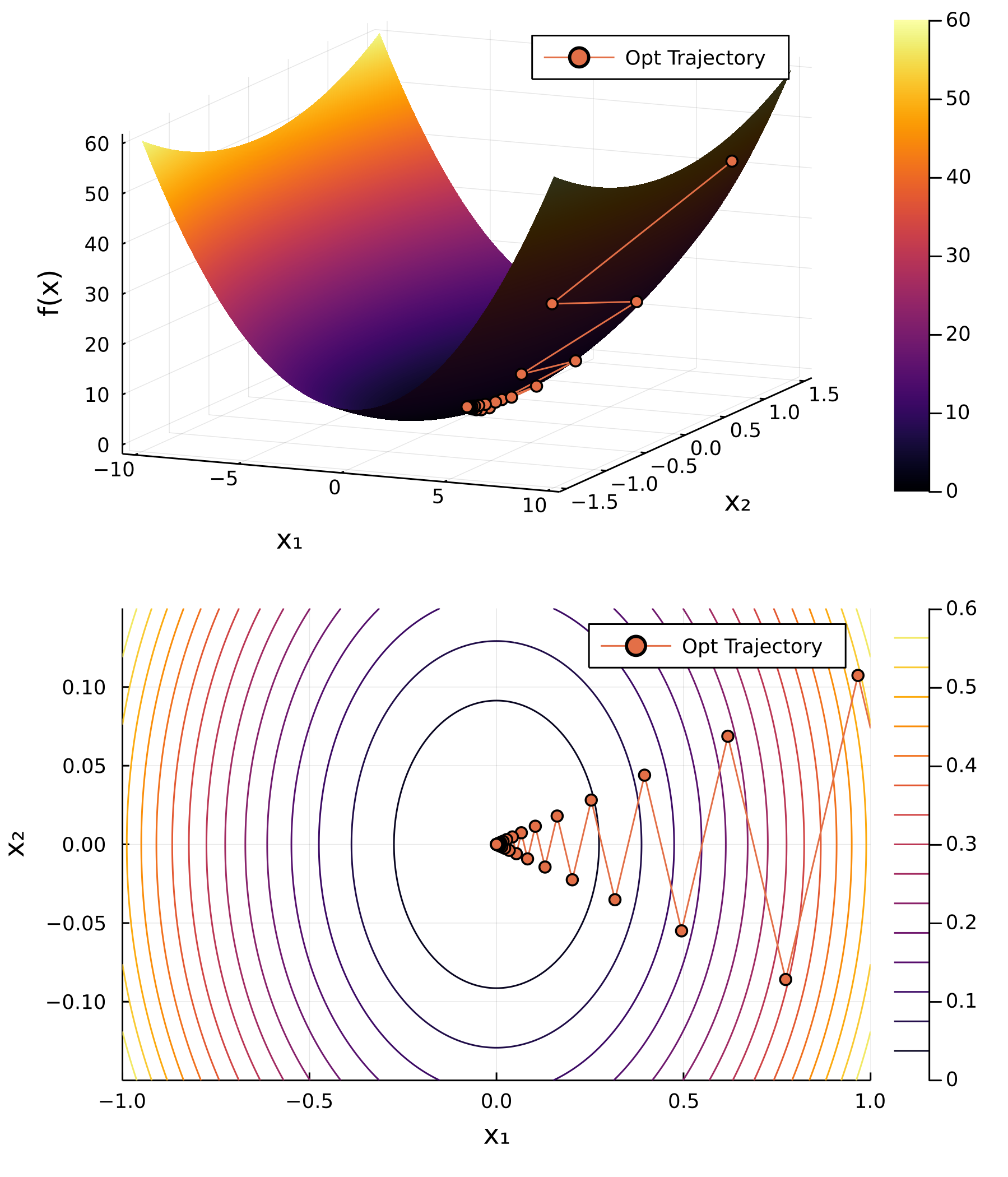
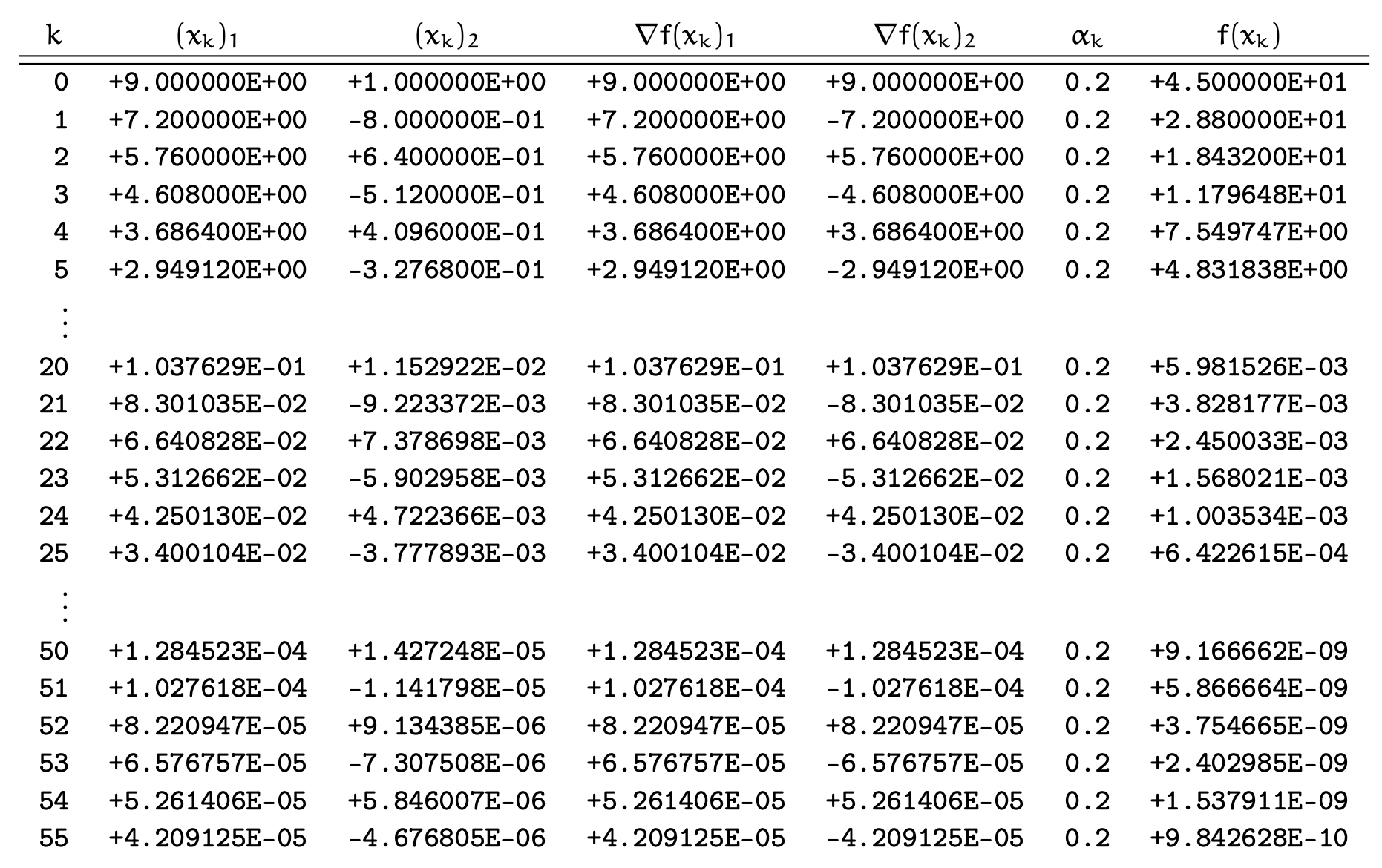
This is very inefficient as we used 56 iterations to optimise this simple parabolic function and only achieved a tolerance of $\epsilon\sim 10^{-5}$. The “zig-zag” phenomenon is very common in gradient descent algorithms due to the anisotropic gradient in each directions. With that said, optimising
$$ f(\mathbf{x})=x_ 1^2+x_ 2^2 \label{eqn:eg2} $$
will not have this problem.
Preconditioning
Now the natural question to ask is, can we turn \eqref{eqn:eg1} into \eqref{eqn:eg2}? We can do so by change of variables
$$ \begin{aligned} &x_{1}^{\prime}=x_{1} \\ &x_{2}^{\prime}=3 x_{2}. \end{aligned} $$
and \eqref{eqn:eg1} can be re-written as
$$ \tilde{f}\left(x^{\prime}\right)=\frac{1}{2} x_ {1}^{\prime 2}+\frac{9}{2}\left(\frac{1}{3} x_ {2}^{\prime}\right)^{2}=\frac{1}{2} x_ {1}^{\prime 2}+\frac{1}{2} x_ {2}^{\prime 2} $$
It is without doubt that in a single iteration, the line search method can find the global minimum, which is $(0,0)$.
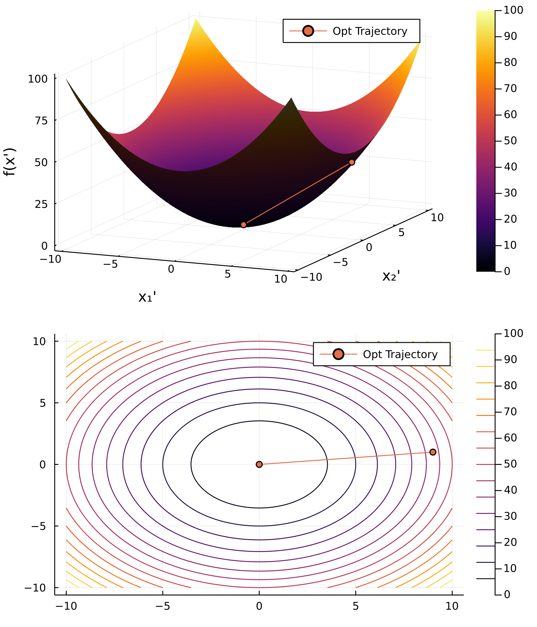
In summary, preconditioning the function makes the original elliptical (anisotropic) contour lines circular (isotropic).
Formally, the preconditioned steepest descent is
$$ \mathbf{x}_ {k+1}=\mathbf{x}_ {k}+\mathbf{H}_ {k}^{-1}\alpha_{k} \mathbf{d}_ {k} $$
where $\mathbf{H}_{k}^{-1}$ is called the preconditioner, which must be symmetric positive definite. We will mention later that, in Newton’s Method, $\mathbf{H}$ is the Hessian of $F$.
Inexact Line Search
Previously, we have performed an exact line search with preconditioning, with analytic gradient and preconditioner. However, these two pieces of information are not always available. In addition, exact line search induces another optimisation over the search path, and may be too computationally expensive to use in practical cases. Often, we use inexact line search instead. Inexact line search tries to “loosely” minimise the function value. In other words, as long as $f(x_{k+1})<f(x_n)$, such step is a “good choice”.
It seems to be a good idea, however, does not necessarily converge. Suppose we want to optimise $y=x^2$ which is simple enough. Let’s try two step sizes which strictly minimise the function value at the next iteration.
- The first choice is $\alpha_k=2+3(2^{-k-1})$. It can be analytically proven that $x_ {k}=(-1)^{k}\left(1+2^{-n}\right)$ and $f(x_ {k+1})<f(x_ {k})$.
- The second choice is $\alpha_k=2^{-k-1}$. It can also be analytically proven that $x_ {k}=1+2^{-n}$ and $f(x_ {k+1})<f(x_ {k})$.
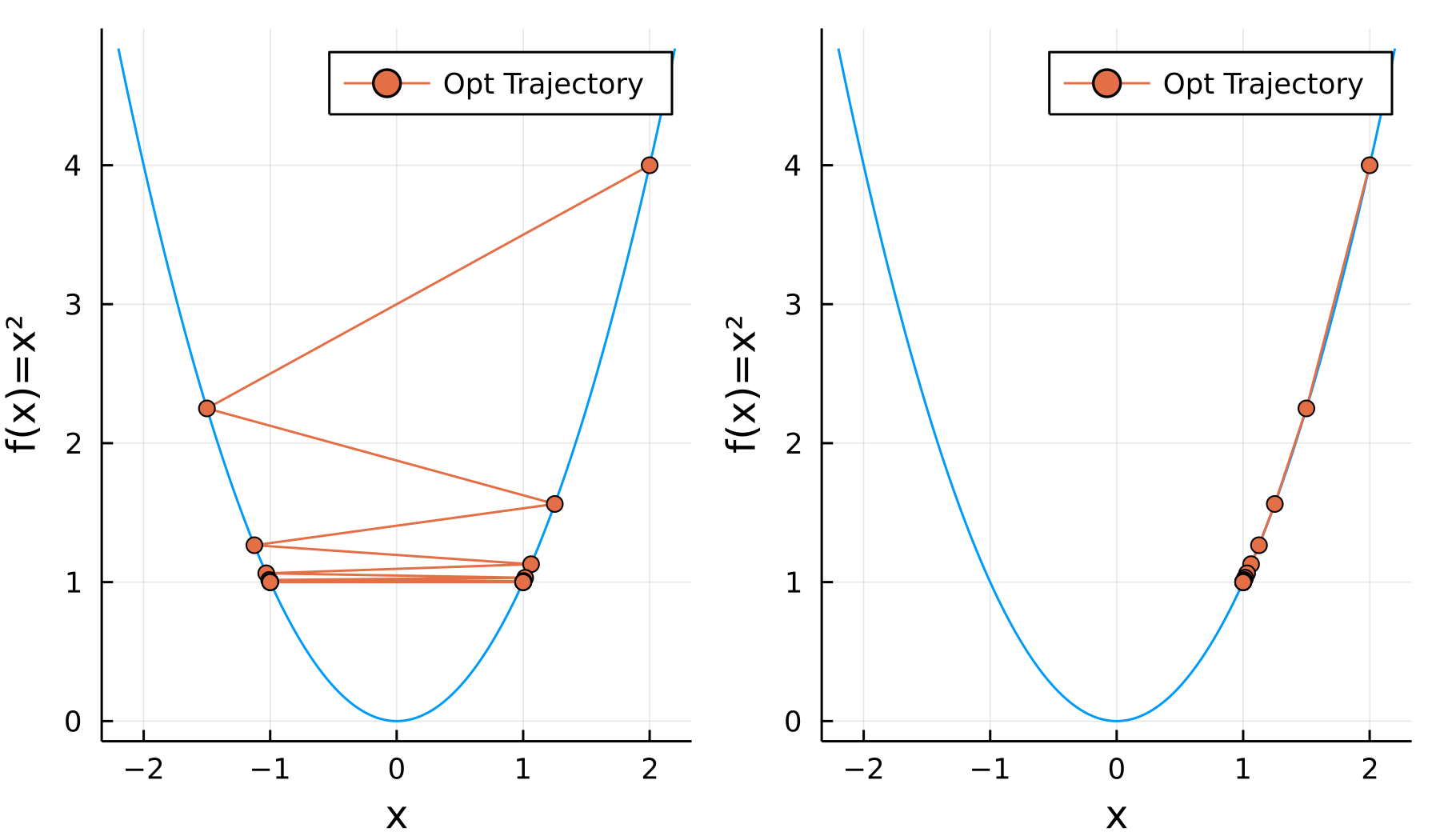
It is clear that for the first case, the function value is monotonically decreasing, however, for the first case, $\lim_{n\to\infty}x_n\nexists$ (does not converge), and for the second case, $\lim_{n\to\infty}x_n=1\neq0$ (converges to a wrong value).
Wolfe Conditions
We want to systematically determine a proper step size instead of randomly guessing.
First Wolfe Condition
We have two ideas of choosing a step size as large as possible.
- If we use a large step, we want a large reduction in function value. \eqref{eqn:wolfe1-1} says, the reduction in function value should be at least proportional to the step size, by the proportionality constant $\gamma$.
$$ f\left(\mathbf{x}_ {k}+\alpha_ {k} d_ {k}\right) \leq f\left(\mathbf{x}_ {k}\right)-\alpha_ {k} \gamma \label{eqn:wolfe1-1} $$
- If we have a large gradient, we want a large reduction in function value. \eqref{eqn:wolfe1-2} says, the proportionality constant $\gamma$ should be proportional to the gradient.
$$ \gamma=-\beta_{1} \nabla f\left(\mathbf{x}_ {k}\right)^{T} \mathbf{d}_ {k},\quad 0<\beta_1<1 \label{eqn:wolfe1-2} $$
Combine \eqref{eqn:wolfe1-1} and \eqref{eqn:wolfe1-2}, we have
$$ f\left(\mathbf{x}_ {k}+\alpha_ {k} \mathbf{d}_ {k}\right) \leq f\left(\mathbf{x}_ {k}\right)+\alpha_ {k} \beta_{1} \nabla f\left(\mathbf{x}_ {k}\right)^{T} \mathbf{d}_ {k},\quad 0<\beta_1<1 $$
It is important to note that both ends of the interval are excluded. Let’s take a look the extreme cases.
- When $\beta_1=0$, we have $f\left(\mathbf{x}_ {k}+\alpha_ {k} \mathbf{d}_ {k}\right) \leq f\left(\mathbf{x}_ {k}\right)$. This is nothing different from the cases we studied previously, and this condition is not sufficient.
- When $\beta_1=1$, we have $f\left(\mathbf{x}_ {k}+\alpha_ {k} \mathbf{d}_ {k}\right) \leq f\left(\mathbf{x}_ {k}\right)+\alpha_ {k} \nabla f\left(\mathbf{x}_ {k}\right)^{T} \mathbf{d}_ {k}$. Note that the RHS is now the tangent line of the function. If the function is convex, it is impossible to find an $\alpha_k$ that satisfies this condition.
- The smaller the $\beta_1$ (less strict), the larger the step size is allowed.
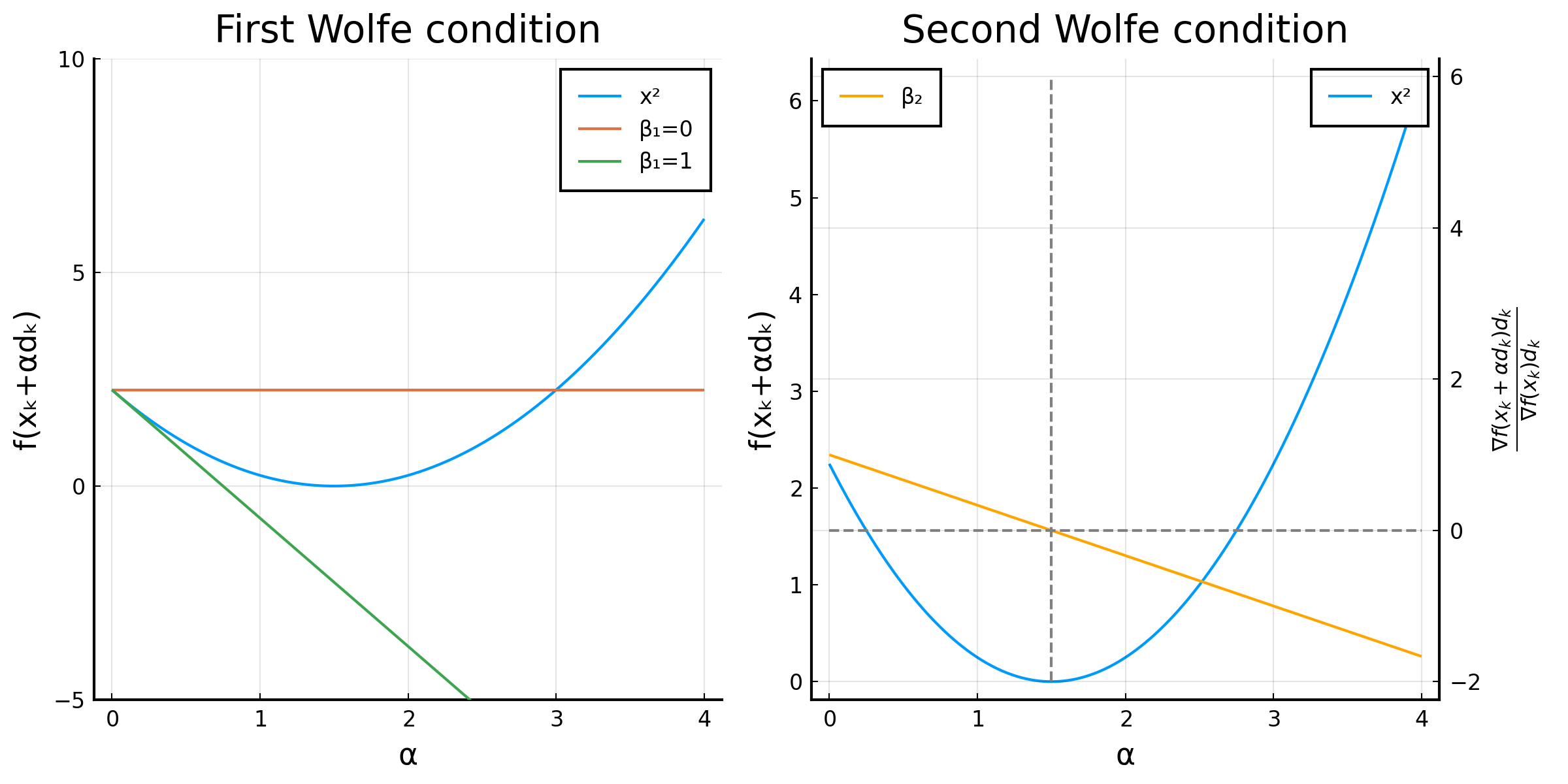
Illustration of first and second Wolfe conditions
This figure shows that, if the starting point is $x=-1.5$, when $\beta_1=0$, $\alpha\le3$, but when $\beta_1=1$, $\alpha\nexists$!
Second Wolfe Condition
The first Wolfe condition avoids a too large step, while the second Wolfe condition avoids a too small step. We define the ratio of the change in directional derivative and the directional derivative itself.
$$ \beta_2=\frac{\nabla f(\mathbf{x} _k+\alpha \mathbf{d} _k)\mathbf{d} _k}{\nabla f(\mathbf{x} _k)\mathbf{d} _k}. $$
When $\alpha=0$, $\beta_2=1$, because there is no movement. When $\alpha=\alpha^*$ so that it reaches the local minimum along the search direction, ${\nabla f(\mathbf{x} _k)\mathbf{d} _k}=0$ because the gradient is perpendicular to the search direction. Consequently, $\beta_2=0$
It is important to note that both ends of the interval are excluded. Let’s take a look the extreme cases.
- When $\beta_2=0$, all step sizes that reduce the function value are accepted.
- When $\beta_2=1$, only the step that reaches the local minimum along the search direction is selected.
It is obvious that, for a sensible selection of $\alpha$, we need
$$ 0<\beta_1<\beta_2<1, $$
called the validity of Wolfe conditions.
Conclusion
This blog briefly introduces the concept of line search and Wolfe conditions. In another blog of this series, we will explore other gradient descent methods, such as Adams, etc..